우선 2단원 내용에 대한 간단한 복습부터 시작
Schrodinger's Equation
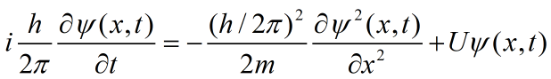
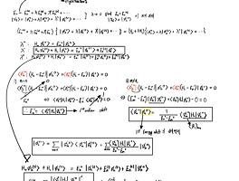
슈뢰딩거 방정식은 wave packet 개념으로 유도 가능
파속을 운동량에 대한 식으로 표현해 (평면파 -> 물질파) 파수 k 대신에 운동량으로 표현
-> 이 때, 원래의 Fourier Transform에는 없는 1/sqrt(hbar) 가 붙어서 새로운 normalization constant 를 만든다.
Wave equation을 x에 대한, 그러니까 위치에 대한 관점으로 보는 경우 <x|Ψ>=Ψ(x)로 나타냄
반면에 p에 대한, 운동량에 대한 관점으로 보는 경우 <p|
Ψ>=Φ(p)로 표현된다. Ψ(x)와 Φ(p)는 Fourier Transform 관계를 가진다. 다만, 원래는 k와 x가 서로 변환이 되는 것
Probability current density J
From Continuity equation.

Lynx: This problem can be solved by getting another Schrodinger's equation. It's about complex conjugate wave equation Ψ*. (From Schrodinger's equation about free particle)
We subtract each other, and we get an equation which form is similar to (4) and we define (2)
<> : Expectation Value(기댓값)
여러 번 측정했을 때의 평균값에 해당
Momentum operator and Displacement operator.
\[x= i \hbar \frac{\partial }{\partial p}\]
\[p= \frac{\hbar}{i} \frac{\partial }{\partial x}\]
in 1D
슈뢰딩거 묘사 vs 하이젠베르크 묘사
슈뢰딩거 방정식은 연산자는 시간에 독립이면서 파동함수가 시간에 따라서 어떻게 변하는 가를, 즉 Ψ(x,t)를 묘사한다. 이를 슈뢰딩거 묘사라 한다.
하이젠베르크 묘사는 파동함수는 시간에 독립이면서 연산자가 시간 종속되는 기술 방법이다.
\[\frac{dA}{dt} = \frac{1}{i \hbar} <[A,H]> + <\frac{\partial A}{\partial t}>\]묘사는 다르나, 이 둘은 같은 Expectation Value를 준다.
How to show operator is Hermitian or Non-Hermitian?
= Go get expectation values for the original and dagger, then, subtract them.
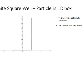
Time-independent Schrodinger's equation.
대표적인 예시는 Infinite Potential Well
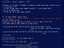
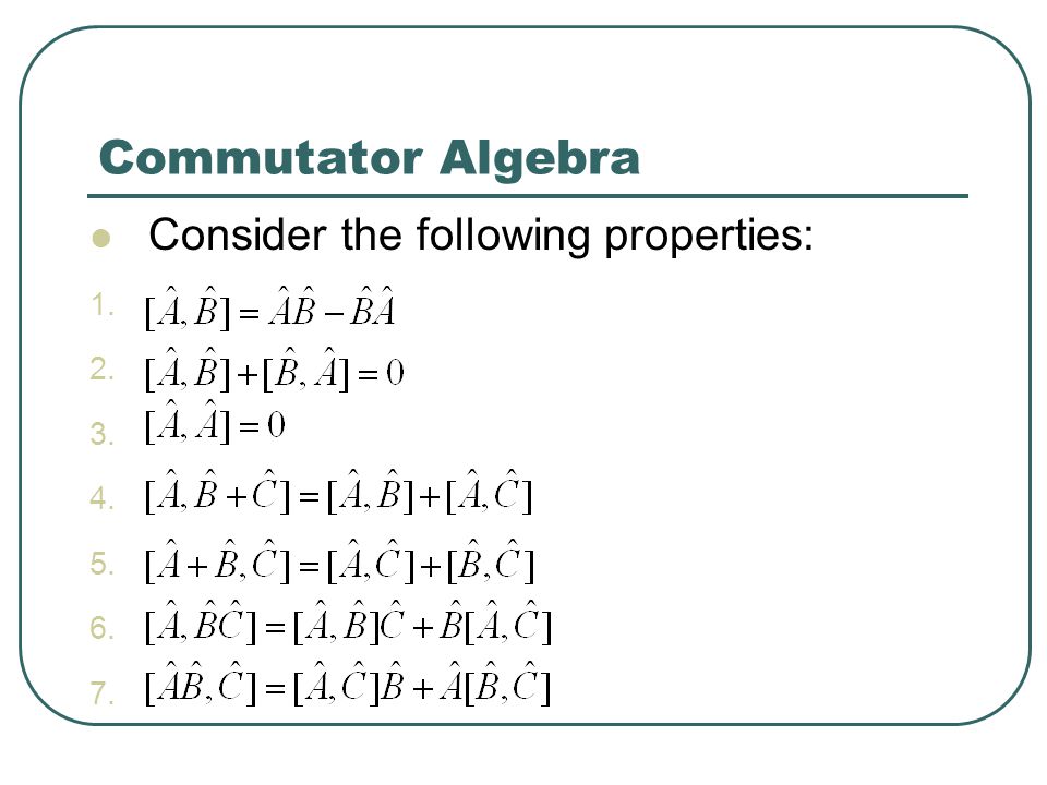
Commutator
Operator A,B에 대해서 AB-BA 는 일반적으로 0이 아님

Commutator 들의 성질을 이용하여 Angular momentum의 각 성분들이 무엇과 Commute 한지 알아낸다.
\[L^{2}\], H(Hamiltonian)과 Commute 한 성질을 가짐을 보일 수 있다.
이 성분들은 Commutator 상에서 Levi-civita notation 을 이용해 간단히 표현
신기하게도 같은 축에서는 non-commute
다른 축에 대해서는 commute (=0)
Commute 하다 = 같은 Eigenfunction을 가진다.
Angular Momentum 에서의 Rasing and Lowering Operator
\[L_{\pm }=L_{x}{\pm }iL_{y}\]
Rasing Opertor \[L_{+}=L_{x}+iL_{y}\] 의 eigenvalue는 [\(m+1) {\hbar}\] 이고,
Lowering Opertor \[L_{-}=L_{x}-iL_{y}\]
의 eigenvalue는 [\(m-1) {\hbar}\]이다.
Operator 들은 행렬로 표시될 수 있음
|1>=\begin{pmatrix}
1\\
0\\
0
\end{pmatrix}
|2>=\begin{pmatrix}
0\\
1\\
0
\end{pmatrix}
...
단 이것들은 모두 Normalize 된 상태, Gasiorowiz p156의 6번 문제를 대표로
Spin
역시 Eigenvalue Problem 이라 10-1은 기존과 같음
10-2 의 Magnetic Moment of spin 1/2 Particles 이 부분에 나오는 magnetic moment 에 대한 내용이 중요.
g : 미세구조 상수
P172 7번
Spin 에 대해서도 각운동량에 대해서와 마찬가지로 똑같은 rotation 규칙이 적용됨을 떠올려서 풀이하면 됨
10번, 쉬움. 그냥 \[e^{x}\] 의 x 자리에 행렬이 들어가는 경우(사실은 이제 수리물리학에서 \[e^{x}\] 는 series 로 정의
출처 : Gasiorowiz Quantum Mechanics, 박환배 양자역학, https://quantummechanics.ucsd.edu/ph130a/130_notes/node214.html
https://en.wikipedia.org/wiki/Baker%E2%80%93Campbell%E2%80%93Hausdorff_formula
Baker–Campbell–Hausdorff formula - Wikipedia
From Wikipedia, the free encyclopedia Jump to navigation Jump to search formula in Lie theory In mathematics, the Baker–Campbell–Hausdorff formula is the solution for Z {\displaystyle Z} to the equation e X e Y = e Z {\displaystyle e^{X}e^{Y}=e^{Z}} fo
en.wikipedia.org
The Commutators of the Angular Momentum Operators
quantummechanics.ucsd.edu
'Quantum Mechanics' 카테고리의 다른 글
| Time independent perturbation theory - 7/9 (0) | 2021.07.14 |
|---|---|
| 7/8 두번째 스터디 (0) | 2021.07.09 |
| Chapter 7. Angular momentum - 개념 (3) | 2021.07.04 |
| Schrodinger's equation in Finite Potential Well (0) | 2021.06.29 |
| Hermitian의 의미 (0) | 2021.04.12 |